2.3 Geometrical opticsAdvanced theoryToday&s geometrical optics (GO) enables to examine the propagation of electromagnetic waves even in complex inhomogeneous media of a given type. As the classical geometrical optics, GO is based on the notion that waves propagate along beams, which can be even curvilinear now. GO is based on the exact mathematical theory coming out Maxwell equations and enabling to compute not only wave trajectories but too variation of magnitude and phase of field intensity and wave polarization. Moreover, the method is well-understandable thanks to the simple notion of beams. As already described in the layer A, theory of geometrical optics is based on the following two assumptions:
In the following, our attention is focused in the media exhibiting a continuous variation permittivity and permeability. The media are assumed to be lossless. Refractive index of the medium
is a real number and is a function of the position (x, y, z). Symbol s denotes the coordinate (curvilinear in general), which is measured along the direction of propagation. Investigating the wave propagation in a homogeneous medium, wave number k = k0(εrμr)1/2 = k0n and the propagation direction are usually known. E.g., the following relation is valid for the field intensity of a plane wave
On the part of the trajectory ds, the phase changes for
In the coordinate system x, y, z, the propagation direction need not to be identical with the direction of a coordinate axis. We usually solve this situation by considering the wave number k as a vector oriented to the propagation direction. Its components kx, ky, kz, to the directions of coordinate axes are wave numbers in the directions x, y, z. In two arbitrarily located points A, B, which coordinates differ for dx, dy, dz, the phases differ for
Geometrical optics does not suppose any a priori knowledge of the direction of wave propagation, because it is different in different points (in the medium of a variable refractive index). In parallel with (2.3B.2), we use
where the distance is not explicitly present. The quantity L is a scalar function of coordinates x, y, z, it is called eiconale and it determines the phase of field intensity in every point. Comparing (2.3A.4b) and (2.3A.2b) shows that on the infinitely short path ds (where n = const), is
Considering (2.3A.4), equation L = const is the equation of a plane, where wave is of the same phase, i.e. the equation of a wave surface. Vector grad L is of the direction of the steepest variation of the eiconale (i.e., even of the phase), and this is the direction of wave propagation. For example: and according to (2.3A.5) is
and therefore
or
As already said in the layer A, the equation
is considered as the basic equation of the geometrical optics. The vector grad L is of the direction of wave propagation in every point, and the curve, which tangent is of the direction grad L in every point, is called beam. Beams can be curvilinear and eqn. (2.3B.8) is the differential equation of beams. For practical calculations, the form (2.3B.8) is inconvenient. Instead, following equations are used:
As already said, s is the coordinate along the beam. Now, the way of deriving the first of relations (2.3B.9) is demonstrated.
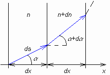
In a homogeneous medium, we exploit in computations the wave number, and we understand it as a vector, which is oriented to the propagation direction. Components of k are kx and ky (in two dimensions) and we can imagine that wave propagates from any point along the pointed trajectory going in parallel to x (wave number kx ) and then, going in parallel to y (wave number ky ). n an inhomogeneous medium, the same approach can be used within a very small region dx, dy only, where the refractive index can be considered constant. In the frame of the whole medium, kx and ky vary, and those variations have to be examined first. In an inhomogeneous medium, computing with refractive index is preferred to computing with wave number. Since k = k0 n and wave number is a vector, even the right-hand side of the equation has to be a vector. Hence, the refractive index n assumed being vector. Its magnitude is n and its direction is identical with the wave propagation (in general, different in different points). Components nx and ny correspond to respective wave numbers, e.g. kx = k0 nx. This formalism converted the inhomogeneous medium to the anisotropic medium, which is not truth from the microscopic point of view. From the macroscopic point of view, this might be considered as a truth: if wave enters the medium in various directions, the trajectory is incurvated different way every time. In the homogeneous medium, the situation is different. Assume a two-dimensional medium, where refractive index varies in the direction x only. In fig. 2.3B.1, two elementary layers of this medium are depicted, including respective quantities. Let us examine variations of components of refractive index nx = n cos(α) and ny = nsin(α) in the direction x:
Rewriting goniometric functions, multiplying, and substituting sin (dα) = dα, cos(dα) = 1 yield
Next, the variation of dny in the direction x, i.e. dny/dx, has to equal zero. This is caused by the fact that two waves propagating along the boundary at different sides near each other have to be of the same wave number, although they propagate in different media. In the opposite case, a continuously rising phase shift between these two waves would exists, and on the boundary, a phase jump would appear, which is impossible. In (2.3B.11b), we put dny = 0, express dα and substitute to (2.3B.11a). We get:
The above relation is rather interesting. It shows that the variation dnx is higher than the variation of the refractive index dn at the same point. The next steps are relatively simple. Eqn. (2.3B.12) is divided by dx and rearranged: dnx/dx = (dnx/ds)(ds/dx) = (dnx/ds)(1/cos(α)). The term cos(α) vanishes and we get the relation (2.3B.9a). Exploitation of (2.3B.9) and (2.3B.10) is demonstrated by the following example. Assume a two-dimensional medium (x, y), where the permittivity ε, and consequently the refractive index n, continuously vary along the coordinate y in accordance with the function n(y); along the coordinate x, the refractive index is constant. Since ∂n/∂x = 0, eqn. (2.3B.9a) results to:
Here, C is an integration constant. Substituting to (2.3B.10), the term containing z is deleted because the task is two-dimensional, and we get
Dividing both equations, the variable s is eliminated and the differential equation of the beam is obtained:
We substitute a given function n(y) and integrated (analytically or numerically). The equation of the beam y = f(x) is the result. The integration constant C is determined using a boundary condition, a known beam direction in a given point. If the value of the eiconale is known in this point LA (A e.g.), we can compute its value in another different point (B e.g.) on the same beam. Using (2.3B.5), we get
if the integration path follows the beam. In our task, the differential ds is replaced by the differential dy according to (2.3B.14), n is replaced by n(y) and integration is performed according toy from yA to yB . [End of example] In layer A, we have found that geometrical optics enables to compute intensity changes during the propagation. This ability is conditioned by the knowledge of computing the shape of beams, i.e. the trajectory of wave. Computation of the intensity is based on the fact that wave energy propagates along beams. This means, that no electromagnetic energy leaves or enters the walls of a tube, which appears when displaying many neighboring beams and which transversal cut gives a closed curve. Energy propagates inside the tube along beams only. On the basis of this idea, the following relation was derived in the layer A:
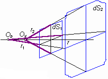
Eqn. (2.3B.17) is not valid for regions, where beams cut (which would cause an infinite field intensity). Such situation appears in a focus and on a caustics. The term caustics is explained thereinafter. Sometimes, beams can exhibit different curvature radii of wave surface in different planes (e.g., astigmatic beams). A part of such a tube is depicted in fig. 2.3B.2. The curvature center of the equiphase surface in the horizontal plane is denoted as Oh, and in the vertical one as Ov. The distances of facet dS1 and Oh (Ov) is r1 (r2), r is the distance between facets dS1 and dS2. Considering fig. 2.3B.2, we get:
Dividing relations, we express the radius of both the facets, and using (2.3B.17), we compute the ratio of intensities. For a homogeneous medium, when respecting phase variation, we get:
The described method of the geometric optics can be used to the examination of the electromagnetic wave propagation through the medium which structure corresponds to the idealized ionospheric layer (if the scaling factor is not considered). Wave radiated by a point source propagates through the medium with the unitary dielectric constant first, and then continues through the layer which dielectric constant decreases down to a certain minimum, and then rises to 1 again. For the given dependency of the dielectric constant in the layer and for the given position of a source, the wave trajectory, the equiphase surface and the eiconale increase can be computed by numeric integration. Below the layer, where several waves are propagating (due to the trajectory curvature), the direction of the propagation, field intensity and eiconale (phase) can be computed for each wave. Computations show that beams return back by nice curls in a certain part of space. Tops of the curls can be connected by an imaginary spline, which is not crossed by any beam, and in a close vicinity of which (below) two neighboring beams intersect. This spline (or a surface in space) is called caustics. |