3.1 WaveguidesDeveloping Matlab
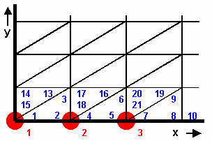 |
| Fig. 3.1D.1 | Two-dimensional finite-element mesh. Blue numbers: local nodes. Red numbers: global nodes |
|
Finite-element method is a general numerical method
for the solution of partial differential equations. Since Maxwell equations,
which describe EM wave propagation in a waveguide, belong to the family of partial
differential equations, finite-element method can be applied to the analysis of
guiding structures.
The basic algorithm of computing field distribution
in a waveguide can be expressed by following steps:
- Waveguide cross-section is divided into finite
elements. If longitudinally homogeneous structure is analyzed, the cross-section
is broken to small triangles. Triangles are called finite elements, vertexes are
called nodes.
- Distribution of the longitudinal component
of electric-field intensity (modes TM) and magnetic-field one (modes TE) is
formally approximated over each finite element by linear, quadratic or cubic function.
Formal approximation is based on unknown nodal intensities and known basis functions.
Each basis function is unitary in a single node and is zero in the rest of nodes.
Approximation is a single equation for N unknown nodal values.
- Formal approximation is substituted to the
solved equation. Due to the proximity, the solved equation is not met exactly.
This fact is represented by adding a residual function to the solved equation.
Decreasing residuum, accuracy of the approximation is increased.
- Residuum is minimized by the method of
weighted residua. The method consists in sequential multiplication of the
residuum by proper weighting functions and in integrating products over the
whole cross-section of the analyzed waveguide. If basis functions corresponding
to the nodes of unknown nodal value are used as weighting functions, we get
N equations for N unknown approximation coefficients.
The described election of weighting functions is called Galerkin method.
- We solve a matrix equation produced by the
Galerkin method. That way, values of unknown nodal intensities are obtained.
In the case of the waveguide, the matrix equation is of the form of generalized
eigenvalue problem. As a result, we get a vector of eigenvalues (vector of
squared critical wave numbers of respective modes) and a matrix of respective
eigenvectors (nodal values of a longitudinal component of field intensity of
respective modes).
- Substituting nodal values to the formal approximation, an approximation
function of the longitudinal component of field intensity over the cross-section
of the waveguide is obtained. On the basis of the longitudinal component
distribution, transversal components of electric field intensity and magnetic
one can be computed.
In practical computations by the finite-element method,
the approach is slightly different. In references, already computed coefficient
matrixes for normalized finite element are at our disposal. We adopt these matrixes,
rearrange them to used finite elements and associate them together with finite
elements to the net. The procedure can be expressed by the following steps:
- Cross section of the waveguide is divided into finite elements, which is
identical with the previous approach.
 |
| Fig. 3.1D.2 | Two-dimensional finite element for linear approximation |
|
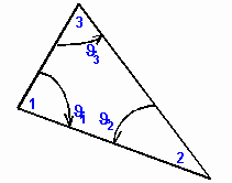
- We find relations for computing coefficients of finite elements. Substituting surface of eth finite element
A(e) and angles at vertexes of eth element (fig. 2) to these relations, we obtain coefficients
for our finite elements. For linear approximation, we get:
|
,
,
,
,
|
( 3.1D.1 )
|
- We build up diagonal matrices for isolated finite elements, i.e. for elements, which are not associated into the mesh
(symbols 0 denote zero matrices of the size 3 x 3)
|
,
|
( 3.1D.2 )
|
- We build up an association matrix, which describes mutual relations among local nodes (blue number is fig. 1)
and global ones (red numbers in fig. 1). Columns of the matrix correspond to global nodes, rows of the
matrix to local ones. If a local node is asked to be associated with a global one, we put 1 to the row of the local node and to the column
of global one. In the opposite case, the matrix element equals to zero. For nodes of fig. 1, the association
matrix is of the following form:
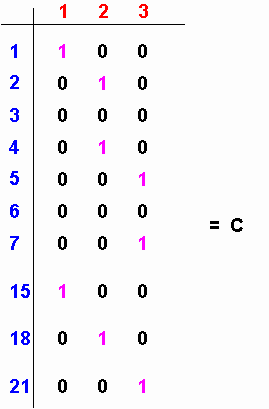 |
| Fig. 3.1D.3 | Association matrix |
|
- Independent isolated finite elements are associated to the finite-element mesh. From the mathematical point of view, the
association is described by the following matrix operation:
|
,
|
( 3.1D.3 )
|
- Solving the final matrix equation (the same equation as obtained by the above-described approach)
we get critical wave numbers of modes k and nodal values of the longitudinal component of electric-field intensity vector E
of those modes. Substituting nodal values to the formal approximation, a global approximation function of the electric-field
intensity component is obtained for every point of the cross-section of the analyzed waveguide.
Our matlab program is based on the presented algorithm. A simplified list of the program follows. Since the source code is in
detail commented, no further description is given.
function kn = linearTE( Nx, Ny);
iNx = Nx + 1;
iNy = Ny + 1;
a = 22.86e-3;
b = 10.16e-3;
dx = ones(1,Nx) * (a/Nx);
dy = ones(1,Ny) * (b/Ny);
Q1 = [ 0 0 0; 0 1 -1; 0 -1 1] / 2;
Q3 = [ 1 -1 0; -1 1 0; 0 0 0] / 2;
Te = [ 2 1 1; 1 2 1; 1 1 2] /12;
N = 2 * Nx * Ny;
St = sparse( 3*N, 3*N);
Tt = sparse( 3*N, 3*N);
n = 0;
for ny=1:Ny
for nx=1:Nx
n = n + 1;
lw = 3*n-2;
hg = 3*n;
St(lw:hg,lw:hg) = Q1 * dx(nx)/dy(ny) + Q3 * dy(ny)/dx(nx);
Tt(lw:hg,lw:hg) = Te * dx(nx)*dy(ny)/2;
St(lw+3*Nx:hg+3*Nx,lw+3*Nx:hg+3*Nx) = St(lw:hg,lw:hg);
Tt(lw+3*Nx:hg+3*Nx,lw+3*Nx:hg+3*Nx) = Tt(lw:hg,lw:hg);
end
n = n + Nx;
end
C = get_c1( Nx, Ny, N)
S = C'*St*C;
T = C'*Tt*C;
clear C St Tt
[H,K] = eig( full(S), full(T));
kn = sqrt( diag( K));
|