4.2 Mutual impedance

Advanced theory

Radiation impedance Z_Σvst on the input port of the antenna can be computed from the value of complex power P_Σ which is radiated by the antenna, when dividing power by input current | I_vst |² of the antenna (eqn. 4.2A.1 in the layer A). Hence, turn our attention to computing the radiated power.

During the process of the radiation of electromagnetic waves, energy delivered to the lossless antenna in free space is transformed to the energy of electromagnetic wave, which propagates in free space, and to the energy, which is periodically exchanged between the antenna and the near field of the antenna. The radiated power P_Σ (complex, in general) can be computed integrating Poynting vector along the closed surface around the antenna. The obtained result is influenced by the selection of the region where the integration is performed.

In the far-field zone (radiation zone), electric field intensity E and magnetic field one H of the radiated electromagnetic wave are in phase. Poynting vector is purely real, and performing its integration along the closed surface (usually a sphere with the center in the antenna), a purely real power P_Σ is obtained. Dividing the power by squared input current I_vst, the real part of the radiation impedance R_Σvst is obtained.

Fig. 4.2B.1

Field intensities on the surface of antenna wire

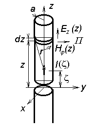
Computing complex radiated power P_Σ, integration of Poynting vector has to be performed in immediate vicinity of the antenna (in case of linear antennas, we integrate along the surface of the antenna wire). Let us start with radiation of a symmetrical dipole of the length 2l and of the radius of antenna wire 2a, which is placed to the coordinate system as depicted in fig. 4.2B.1. On the surface of the cylindrical antenna wire, the current I(z) excites a longitudinal component of electric field intensity E_z(z) and a transversal tangential component of magnetic field intensity H_φ(z).

Magnetic field intensity H_φ(z) on the surface of a relatively thin wire is primarily determined by the current I(z) in the immediate vicinity of the element dz. Applying Amper low, we get

H_{φ} (z) = \frac{I (z)}{2 π a}

( 4.2B.1 )

Electric field intensity E_z(z) on the surface of the antenna wire can be expressed in term of vector potential A_z(z) considering a known current distribution I(z)

A_{z} (z) = \frac{μ}{4 π} \int_{- l}^{l} I (ζ) \frac{e^{- j k r}}{r} d ζ

r = \sqrt{{(z - ζ)}^{2} + a^{2}}

( 4.2B.2 )

Electric field intensity E_z(z) equals then to

E_{z} (z) = - j ω (A_{z} + \frac{1}{k^{2}} g r a d_{z} d i v (A_{z})) = - j ω (A_{z} + \frac{1}{k^{2}} \frac{\partial^{2} A_{z}}{\partial z^{2}})

( 4.2B.3 )

If the radius of the antenna wire a is significantly smaller than its length 2l, and if radiation of the wire ends is neglected, Poynting vector is of the radial component only

Π = - E_{z} (z) H_{φ}^{*} (z)

( 4.2B.4 )

An element of the wire surface dS = 2π and dz radiates then the power

d P_{Σ} = Π 2 π a d z = - E_{z} (z) I_{z}^{*} (z) d z

( 4.2B.5 )

where asterisk denotes complex conjunction.

Complex power radiated by the whole antenna P_Σ is obtained integrating along the whole dipole

P_{Σ} = \int_{- l}^{l} d P_{Σ} = - \int_{- l}^{l} E_{z} (z) I_{z}^{*} (z) d z

( 4.2B.6 )

Components of radiation impedance Z_Σvst on the input port of the antenna can be obtained when dividing the power P_Σ by squared input current I_vst

Z_{Σ v s t} = - \frac{1}{{| I_{v s t} |}^{2}} \int_{- l}^{l} E_{z} (z) I_{1}^{*} (z) d z

( 4.2B.7 )

The described approach is formally simple, but solving a given problem, evaluation of integrals is rather problematic. The main advantage of this approach is given by the possibility to compute impedances of elements in an antenna array as shown in the layer A.

Now, turn our attention to a small detail of the approach. We should disagree with the orientation of the vector Π in fig. 4.2B.1, which does not correspond to the clockwise system E x H. Moreover, the cause of the sign "minus" in eqn. (4.2B.4) is not clear. Maybe, we may argue that the opposite orientation and the opposite sign can mutually compensate. Next, the reader can ask why antennas are fabricated from well-conductive metals: using perfect conductors, tangential component of electric field intensity vanishes, value of Π is zero and such a perfect antenna does not radiate. Hence, more detailed attention to the above-described approach is demanded.

Let us start with the zero tangential electric field component and assume perfect conductivity of the antenna wire. If our computations consider an exact current distribution then zero tangential electric field component is obtained everywhere on the surface of the antenna wire except of the infinitesimally short excitation gap at z = 0. Understanding Poynting vector as a surface power density, antenna seems to radiate in the excitation gap only.

Finite conductivity of real metals does not change anything on this fact. Tangential component on the surface is not indeed zero, but the real power penetrating inside the conductor is relatively small (this power is converted to heat in the conductor). The only region, where real component of Poynting vector is directed out of the antenna, is the feeding gap.

This conclusion seems to be rather surprising and might to invoke doubts. At least, this conclusion does not correspond to the notion of an antenna as a set of radiating elementary dipoles. Fortunately, these problems can be relatively simply solved.

First, nothing proves the fact that the antenna radiates in the feeding gap only. Poynting theorem says only that integrating the product E_t(z) H(z) along the closed surface equals to the total incoming power. Meaning of the surface power density is only attributed to this product because it can be usually done. Therefore, no contradiction with respect to the theory is revealed. Moreover, there is no need for asking the question where the power is radiated, and the so-far notions can be kept.

Even from the mathematical point of view, no serious problems appear. Due to the practical reasons, computations are not performed with an exact current distribution I(z) but with the approximate one I'(z) (of sine nature, usually). Even a small difference between I(z) and I '(z) causes the tangential component of electric field intensity to differ from zero on the surface of the antenna wire, and the integral (4.2B.6) can be evaluated. Computations can be therefore performed using an approximate current distribution I'(z). Satisfactory correctness of the approach can be proven following A. A. Pistolkors:

Fig. 4.2B.2

Substition of antenna feeding for current distribution I'(z)

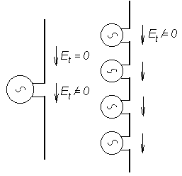
The real antenna (symmetric dipole) is depicted in fig. 4.2B.2a. The antenna is fabricated from a perfect conductor, the current distribution is given by I(z) and on the whole surface (except of the excitation gap) the tangential component of electric field intensity equals to zero. Since an approximate current distribution I'(z) is considered in computations, E_t differing from zero is obtained, and consequently, a certain radiated power is computed.

In order to prove the computed power being approximately equal to the really radiated power, we can imagine to analyze an imaginary antenna of the same shape and the same dimensions as the real antenna but of I'(z) as an exact current distribution. Then the imaginary antenna has to be fed by a different way. We have to admit the excitation consisting of a vertical row of elementary sources (fig. 4.2B.2b), which voltages are set to enforce the current distribution following the function I'(z). The fact that the tangential component of electric field intensity is non-zero on the surface of the imaginary antenna is correct because the whole surface of the imaginary antenna is covered by excitation gaps. The power we have computed is valid for our imaginary antenna. If the difference between I(z) and I'(z) is small, then the computed power approaches the power radiated by the real antenna.

Finishing our discussion, we can go back to the basic idea.

In the set of parallel dipoles (fig. 4.2A.1 in the layer A), the power radiated by the first element of the array is expressed first. The total electric field intensity E_z1(z) on the surface of the first element equals to the sum of contributions of all the elements of the array

E_{z 1} (z) = E_{11} (z) + E_{12} (z) + \dots \dots + E_{1 n} (z)

( 4.2B.8 )

Power P_Σ₁ radiated by the first element is obtained when substituting to eqn. (4.2B.6). Formal rearrangement yields the relation

\begin{array}{l} P_{Σ 1} = - \int_{- l}^{l} [E_{11} (z) I_{1}^{*} (z) + E_{12} (z) I_{1}^{*} (z) + \dots \dots + E_{1 n} (z) I_{1}^{*} (z)] d z = \\ = I_{v s t 1}^{*} [- I_{v s t 1} \int_{- l}^{l} \frac{E_{11} (z)}{I_{v s t 1}} \frac{I_{1}^{*} (z)}{I_{1 v s t}^{*}} d z - I_{v s t 2} \int_{- l}^{l} \frac{E_{12} (z)}{I_{v s t 2}} \frac{I_{1}^{*} (z)}{I_{1 v s t}^{*}} d z - \dots \dots - I_{v s t n} \int_{- l}^{l} \frac{E_{1 n} (z)}{I_{v s t n}} \frac{I_{1}^{*} (z)}{I_{1 v s t}^{*}} d z] \end{array}

( 4.2B.9 )

Integrals

Z_{j k} = \int_{- l}^{l} \frac{E_{j k} (z)}{I_{v s t k}} \frac{I_{j}^{*} (z)}{I_{v s t j}^{*}}

( 4.2B.10 )

are called mutual impedances and are given in Ohms. Thanks to the formal rearrangement, integrals (4.2B.10) do not depend on the magnitudes of currents in antenna elements because the field intensity E_jk excited on the surface of j-th element by the radiation of k-th element is proportional to the current I_{vst k} in k-th element of the antenna array.

For parallel dipoles, results of the integration in (4.2B.10) are expressed in the form of tabulated functions (integral sine, integral cosine). In order to get numerical values of mutual impedance components Z_jk, computer program described in the layer C can be used. Results describe coupling between the couple of parallel dipoles of the same length 2l, which is related to the maximal current I_max. Values Z_{jk vst}, which are related to the input current of the dipole, are obtained performing re-computing according to eqn. (4.2A.4) in the layer A.

Dependency of the magnitude of the components of mutual impedance on the distance between dipoles was already demonstrated in the layer A (fig. 4.2A.2) for the couple of parallel symmetric dipoles with a standing current way. Negative values of the mutual impedances R_jk and X_jk express the fact that for a given spatial arrangement, radiation of k-th element reduces the magnitude of real or imaginary part of the power P_Σ_j which is radiated by j-th element of the antenna array. Decreasing magnitude of mutual impedance for long distances corresponds to the decrease of the electric field intensity E_jk for increasing distance.

Exploiting eqn. (4.2B.10), self-impedance of a stand-alone antenna element Z_jj can be computed if the distance between elements d is set to the value of the radius of the antenna wire a. This approach corresponds to the situation described when deriving eqn. (4.2B.7): we considered electric field intensity on he surface of j-th antenna wire E_jj excited by a current flowing through the axis of the same wire.

The method of induced electromotoric forces enables to compute the radiated power, and consequently the values of mutual impedances even in the case of non-parallel antenna wires. Then, we have to respect a different spatial orientation of vectors of electric field intensity E_jk with respect to the surface of j-th antenna wire. Decomposing vector E_jk to respective components and exploiting more general expression for the power contribution dP_Σ, we obtain formally more complicated relations. That way, coupling between crossed wires of a turnstile antenna and further situations can be solved.