4.6 Multi-band patch antennasComputer simulation
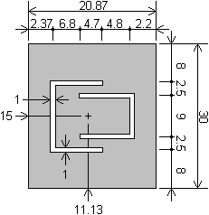
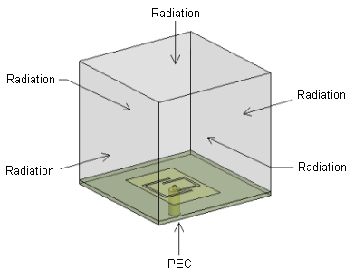
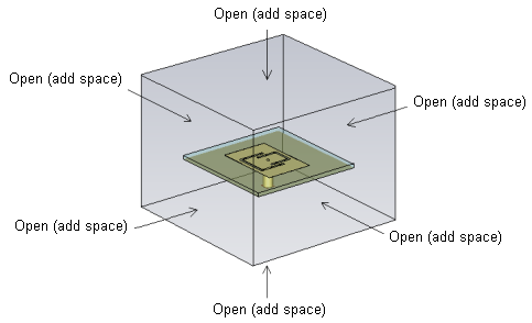
In this layer we are going to learn how to model planar antennas in the modern commercial softwares Ansoft HFSS and CST Microwave Studio. The first one, similarly to Comsol Multiphysics, is based on finite element method (FEM), and the second one uses the finite integration technique (FIT). The FIT is very similar to finite difference time domain (FDTD) method. The main difference is that FDTD solves differential Maxwell’s equations, while FIT uses their integral form [35], [36]. Let us consider a planar antenna with the metallic patch from fig. 4.6B.2. The patch is placed on dielectric substrate Arlon AD600 with relative permittivity εr = 6.15, thickness h = 1.575 mm and dimensions 50x50 mm2. The antenna is fed by coaxial probe. A simple Matlab code for calculating the approximate size of patches is introduced in layer C. Parameters of the antenna after final tuning in Ansoft HFSS are summarized in fig. 4.6B.2. The antenna was tuned manually and the surface current distribution was monitored. In such a way we successfully obtained good impedance matching (S11 < –10 dB) near to required frequencies 2.45 GHz and 3.60 GHz. Together with the results from Ansoft HFSS, computer simulations of the antenna also from CST Microwave Studio are introduced and mutually compared in the next section. In fig. 4.6B.2 the computer model (together with the applied boundary conditions) of the antenna under investigation in the selected two softwares is depicted. In both cases, finite substrate and finite ground plane are considered.
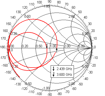
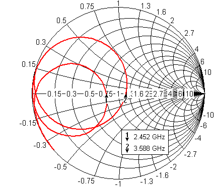
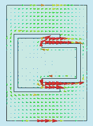
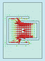
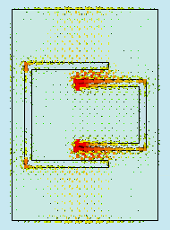
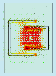
Let us now investigate the frequency dependence of the input impedance of the antenna (fig. 4.6B.3). Clearly, resonant frequencies computed by Ansoft HFSS are f1 = 2.439 GHz and f2 = 3.600 GHz, and the ones calculated by CST Microwave Studio are f1 = 2.452 GHz and f2 = 3.588 GHz. Because of the resonant frequencies obtained by different programs are in good agreement, our computer models seem to be correct. Fig. 4.6B.3 shows the surface current density on the metallic patch of the antenna. The results are the same as computed in Comsol Multiphysics – at the lower resonant frequency currents flow on the whole patch, whereas at the higher resonant frequency only in the area bounded by the U slots.
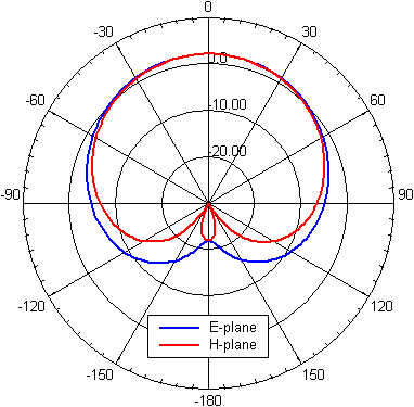
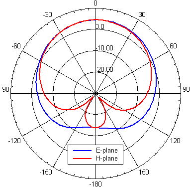
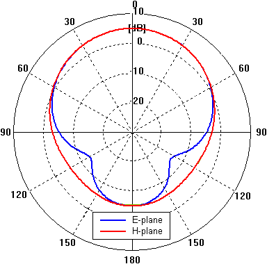
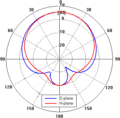
Radiation patterns of the designed antenna are shown in fig. 4.6B.5.
Now the properties of our antenna are described completely. Comparison of the results from the two softwares follows. A simple dual-band planar antenna was modeled in Ansoft HFSS and CST Microwave Studio. The first of the softwares solves Maxwell’s equations using FEM, the second one uses FIT. In both cases the antenna was placed on finite dielectric slab and finite ground plane with dimensions of 50x50 mm2. Resonant frequencies obtained by different programs agree well and the surface current density corresponds to the one computed in Comsol Multiphysics. Small differences in radiation patterns computed by the two programs are probably caused by slightly different boundary condition setup as seen in fig. 4.6B.2. Comparing the radiation patterns for E-plane and zero elevation at 2.45 GHz and 3.60 GHz, larger beamwidth at the higher resonant frequency can be observed. This indicates the existence of surface waves. At higher frequencies when thickness of the substrate becomes comparable with the wavelength, strong excitation of surface waves can lead to their diffraction at edges of finite dielectric slab and deform the radiation pattern. | ||||||||||||||||||||||||||||||||||||||||||||||||