Multimedia textbook

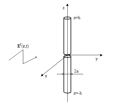
5.1 Time-domain modeling of wire antennas by method of moments

Basic theory

In the chapters 4.1, 4.4, and 4.5 the wire dipole, microstrip dipole and patch antenna are modeled by method of moments in the frequency domain. The integral equation is transformed to the system of algebraic equations and the current distribution on the antenna is computed at the steady harmonic state at the given frequency. The antenna parameters can be computed from the current distribution.

Numerical modeling of antennas in the frequency domain is effective if the antenna parameters are desirable in the narrow band of frequencies. If the wideband analysis is desirable, it is better to use time-domain analysis. However, this one is suitable only for the structures with low Q-factor, otherwise, the computed response is too long, and the analysis is time consuming.

The basic principles of the time-domain modeling of wire antennas will be described in this chapter. Again, as in the frequency domain, the formulations which come out from Maxwell’s equations in the differential or integral form are solved. In this chapter we focus our attention on the integral formulation, as in the chapters 4.1, 4.4 and 4.5.

The integral formulation in the time domain is more complicated than in the frequency domain due to the time derivative of the vector potential, thus, the integro-differential formulation is solved instead of the pure integral formulation.

Due to the education purpose of this chapter, we focus our attention only on the solution of the symmetric wire dipole, because the solution of more complicated structures is, from the point of the derivation and implementation, more demanding.

Time-Domain Modeling of Wire Dipole by Method of Moments

For modeling a symmetric wire dipole in the time domain we come out from a similar situation as in case the frequency domain. Let’s suppose that the symmetric wire dipole is made from the perfect electric conductive material, and placed in the vacuum. The dipole axis is identical with z axis of the cylindrical coordinate system, and the electromagnetic plane wave incidents on it (fig. 5.1A.1). The intensity of the electric field is parallel to z axis, and the waveform is arbitrary. Further, the wire radius a is much smaller than the wavelength.

Fig. 5.1A.1

Wire dipole placed along the z axis and excited by electromagnetic wave.

The incident plane wave E^I induces a current I_z (the dipole is placed along z axis) on the dipole surface. Since at open ends of the antenna the electric currents do not have a chance to flow, the electric charge σ accumulates. In the next instants the accumulated charge flows off and in, depending on the phase of each spectral component of the incident wave. The induced currents and charges become the sources for the radiation of the secondary wave. The influence of the current along the z axis can be described by the vector potential [37]

A_{z} (z, t) = \frac{μ}{4 π} \int_{ξ = - h}^{h} \frac{I_{z} (ξ, t - R (z, ξ) / c)}{R (z, ξ)} d ξ

( 5.1A.1 )

The influence of the charge density can be described by the scalar potential

φ (z, t) = \frac{1}{4 π ε} \int_{ξ = - h}^{h} \frac{σ (ξ, t - R (z, ξ) / c)}{R (z, ξ)} d ξ

( 5.1A.2 )

The value of the vector potential A_z at a arbitrary “target” point z, and instant t can be computed by the addition of contributions of the current components from all “source” points ξ on the antenna axis. The source current has to be retarded about time R/c which the wave needs for traveling the distance between the source ξ point and the target point z

R (z, ξ) = \sqrt{a^{2} + {(z - ξ)}^{2}}

( 5.1A.3 )

Further, c in (5.1A.1) is speed of light in the given environment. The contribution to the vector potential is not proportional to the distance between the source and target point. The integration has to be carried out along the whole antenna structure. Finally, the value of the integral is multiplied by the permeability of surrounding medium μ (the vacuum).

In case of the scalar potential, the current distribution is replaced by the charge density σ. The result of the integration is, instead of the multiplication by the permeability, divided by the permittivity of the surrounding medium ε. The rest in the equation (5.1A.2) stays the same as in (5.1A.1).

Since the current and the charge are mutually tied, the relations (5.1A.1) and (5.1A.2) has to be tied by the continuity equation

\frac{\partial σ (z, t)}{\partial t} = - \frac{\partial I_{z} (z, t)}{\partial z}

( 5.1A.4 )

If the vector and scalar potentials are known, the intensity of the electric field radiated by antenna E_z^S (the scattered field) can be computed

E_{z}^{S} (z, t) = - \frac{\partial ​ A_{z} (z, t)}{\partial t} - \frac{\partial φ (z, t)}{\partial z}

( 5.1A.5 )

The derivative of the vector potential with respect to time describes “the dynamic contribution” of the electric charge on the antenna to the radiated wave (the electric currents, charges in motion, are the source for the vector potential). The partial derivative of the scalar potential with respect to the variable z express the “static contribution” of the electric charge on the antenna to radiated field (the static charges, accumulated at ends of the antenna, are the source for the scalar potential)

On the surface of the perfect electric conductor the intensity of the electric field has to satisfied the boundary condition

E_{z}^{S} (z, t) + E_{z}^{I} (z, t) = 0

( 5.1A.6 )

The system of equations (5.1A.1) to (5.1A.6) is solved numerically in two steps. The first one consists in the space discretization of the problem and the second one consists in the application of time algorithms on the result of the first step.

The first step is analogical to the solution in the frequency domain, where the method of moments is used for the “transformation” of the integral equation to the system to algebraic equations. Here, we use again the method of moments for the “transformation” of the integro-differential equation (5.1A.5) to a system of the retarded differential equations (the space discretization of the problem).

For the second step (the application of the time algorithms), it is possible to use either the explicit, or the implicit algorithm. At the explicit one, the length of the time step Δt has to satisfy the following condition: Δt ≤ R_min/c, where R_minis the smallest distance of centers of the discretization elements and c is the speed of the light in the surrounding medium. At the implicit algorithm, the length of the time step can be chosen arbitrary. The larger length of the time step increase the speed of computation, but the accuracy falls down. These approaches belong to the marching on in time (MOT) methods.

The marching on in order method (MOO) is the next method. It is based on the approximation of the transient response by a set of weighted Laguerre polynomials. The advantage of MOO is its unconditional stability, but the disadvantages are the higher demands on the implementation, and less effectiveness in the comparison to MOT.

Due to above facts, we focus our attention on MOT. Although we mentioned that the system of equations (5.1A.1) to (5.1A.6) is solved in two steps (the space discretization and the application of time algorithms), we will merge both these steps. It is appropriate to notify that by MOT the system of retarded differential equations is transformed to the system of difference equations (the derivative of the vector potential with respect to tome (5.1A.5) is replaced by appropriate difference).

The advantage of the explicit algorithm is its easier implementation and there is no need to compute an inverse matrix as in case of the solution in the frequency domain, or as at the implicit approach. However, the explicit approach suffers often from the late time oscillation (the computed response is not steady, but grows exponentially.). Therefore, the attention in this chapter is focused only on the implicit approach.

Excitation pulse

Before, than we focus our attention on the implicit approach, let’s choose an appropriate excitation pulse.

If we chose the Dirac pulse, the spectrum of the excitation signal would be equally spread over the infinite frequency domain. Since in the technical practice the solution is desirable over the limited bandwidth and we do not have unlimited computer memory and the power of a computer, thus, the Dirac pulse is not an ideal choice.

Instead of the Dirac pulse it is better to use the Gaussian pulse modulated by a harmonic signal. By change of its parameters, it is possible to analyze only the band of our interest.

The vector of the intensity of the electric field of the Gaussian excitation pulse modulated by harmonic signal is given

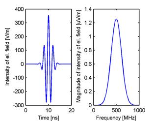
E^{I} (r, t) = E_{0} \frac{4}{c T \sqrt{π}} \exp [- {(\frac{4}{T} (t - t_{0} - \frac{r \cdot a_{k}}{c}))}^{2}] \cos (2 π f_{0} t)

( 5.1A.7 )

where E₀ is the vector of the intensity of the electric field of the excitation wave at the origin of the coordinate system, r is the positional vector of the point where the intensity of the excitation wave is computed, a_k is the unit vector in the direction of the propagation, c is the speed of the light in the surrounding medium, T is the width of the Gaussian pulse, t₀ is the retardation of its peak, and f₀ is the center frequency of the analyzed band. The example of the Gaussian pulse modulated by the harmonic signal with its spectrum, defined by the following parameters: |E₀|=120π V/m, T=8 ns, t₀=10 ns and f₀= 500 MHz, is depicted in fig. 5.1A.2.

Fig. 5.1A.2

Gaussian pulse modulated by harmonic signal in time (leftside) and frequency (rightside) domains.

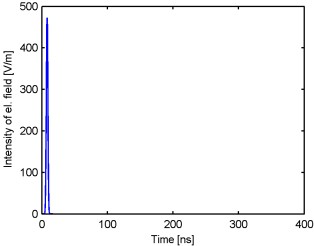
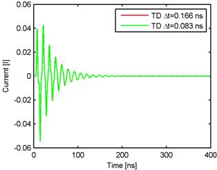
Implicit algorithm

The derivation of the implicit algorithm is demanding (the system of the equations (5.1A.1) to (5.1A.6) is discretized in space and time), and for the interested reader it is carried out in the layer B. In this layer the properties of the implicit scheme are only discussed.

At the implicit algorithm, opposite to the explicit one, the inverse matrix has to be solved and its implementation on the computer is more demanding than in case of the explicit algorithm. However, its advantage is that the length of the time step can be chosen arbitrarily (we should keep in mind, the length of the time step influences the accuracy), and this algorithm is more stable than the explicit one.

Using the implicit algorithm will be demonstrated on the analysis of the wire dipole of the length 2 m, which is excited at its center by the Gaussian pulse modulated by a harmonic signal (5.1A.7) defined by the following parameters: E₀=120π V/m, T=6 ns, t₀=8 ns, f₀ = 0 Hz. Since the center frequency of the analyzed band is 0 Hz, let’s further call this pulse as the Gaussian pulse. Let’s chose the length of time analysis 400 ns. The body of the dipole is divided to 40 segments (the space discretization of the task, layer B). The analysis is carried out two times for different lengths of the time step. In case of the first analysis the length of the time step is Δt = R_min/c = 0.166 ns, cΔt = 0,05 m, and in the case of the second analysis the length of the time step is half of the first case, Δt = R_min/(2c) = 0.083 ns, cΔt = 0,025 m (the time discretization of the task).

The excitation Gaussian pulse is depicted in fig. 5.1A.3. The computed current responses to this pulse at the center of the dipole are depicted in fig. 5.1A.4. Comparing both figures it can be said that the computed responses are significantly larger than the excitation pulse and the difference between computed current is very small.

The wire dipole is a narrow band antenna which is able to “transform” the energy to the free space only within the limited range of the frequencies. Since the excitation pulse carries the energy even at the frequencies, where the antenna has this ability significantly smaller, the energy goes from the one arm of the dipole to the other and back, and the energy is gradually radiated.

Fig. 5.1A.3

Excitation Gaussian pulse.

Fig. 5.1A.4

Current responses on the Gaussian pulse (obr. 5.1A.3) in the center of the wire antenna for different lengths of the time step

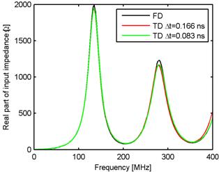
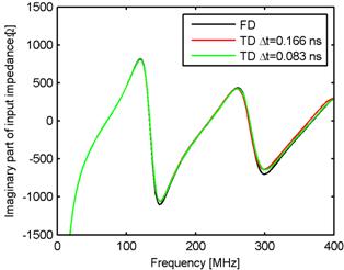
Since the computed responses are stable, the input impedance of the wire antenna can be computed (fig. 5.1A.5, denoted by TD). In the same picture the input impedance computed by the method of moments in the frequency domain is depicted (denoted by FD). The solution in the frequency domain is taken as the reference solution because its accuracy is known. Comparing this solution with the results for the implicit algorithm for the length of the time step Δt = R_min/c = 0.166 ns, cΔt = 0,05 m (red line) we can say that larger differences are apparent at higher frequencies. These differences are mainly caused by the discretization of the system of the equations (5.1A.1) to (5.1A.6) in time. If we decrease the length of the time step to the half of the original value (green line), the differences are smaller (more accurate approximation in the time). The length of the time step influences the accuracy of the algorithm.

Fig. 5.1A.5

Real (left) a imaginary (right) part of the input impedance of the analyzed wire dipole.

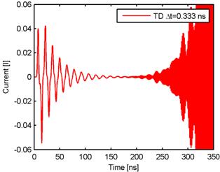
The length of the time step influences the stability of the algorithm too. This fact is demonstrated in fig. 5.1A.6, where the current response of the same dipole antenna for the double length of the time step (Δt = 2R_min/c = 0.333 ns, cΔt = 0,1 m.) is depicted. The computed response is not stable, but it grows to infinity.

Fig. 5.1A.6

Unstable current response to the Gaussian pulse (fig. 5.1A.3) in the center of the wire dipole (larger length of the time step).

For stabilizing the time algorithm different techniques can be used, however, these ones are behind the scope of this chapter.