6.1 Analysis of frequency selective surfacesMatlab program
 |
| Fig. 6.1C.1 | GUI of the program in Matlab |
|
Spectral domain moment method is implemented in the computer program for analysis frequency selective surfaces
(FSS) with the rectangular patches. This program is composed from the several separated m-files. These m-files
are called after setting input parameters and after request for the computation. The N-dimensionals Matlab arrays
and the nested loops are used. Program is controlled from user friendly GUI interface.
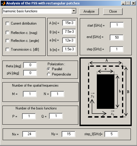
Program Description
The computer program for analysis frequency selective surfaces with rectangular patches can computes the magnitude
and the angle of the reflection coefficient, transmission coefficient in decibels and the current distribution on
the conductive patches. The spectral domain method for the computing these parameters is used. For the approximation
of the current distribution are available two types of the basis functions in Popupmenu at the top of the window (fig. 6.1C.1).
The main window includes Edits for entering the dimensions of the cells and for the dimensions of the conductive patches.
Meanings of the parameters are illustrated on the picture, which represents the cell and the patch of FSS. At the right
side of the window are Edits for the setting the step and the interval of the frequencies, which will be used for the analysis.
The program enables setting the perpendicular or the parallel polarization and the angles of the incidence (theta and phi are
common angles in the spherical coordinates). The Edits named as M, N denotes the numbers of the harmonics for spatial frequencies
in the directions x and y, respectively. Another Edits named as P, Q are for entering the level of the basis functions. At the
bottom of the window are Edits for the setup the depiction of the current distribution. The parameter Nx and Ny sets the density
of the depiction and the parameter named as Step_I is step of the frequencies for which is the current distribution depicted.
When we have set all these parameters we can choose the required parameter by the Checkboxes and click on the button Analyze.
The program is closed by the click on the button Close.
Results of the Analysis
In this section the frequency selective surface with rectangular patches is analyzed with the program in the Matlab and with the ANSOFT Designer.
The results of analyses and the computing times are compared.
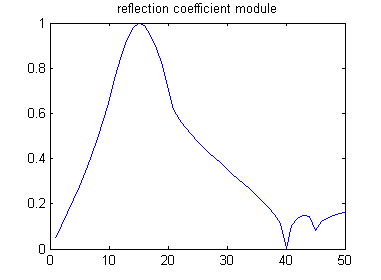
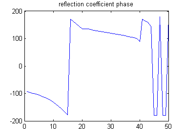
The conductive patch is of the dimensions a = 12 mm, b = 1.5mm, the cell is of the dimensions A = 15 mm, B = 7.5 mm.
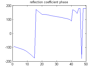
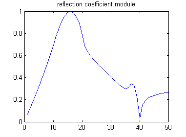
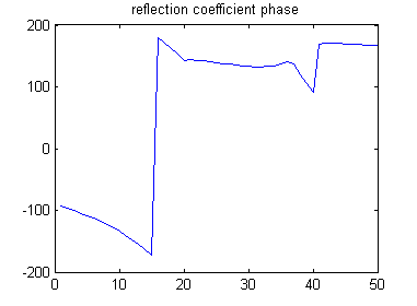
Magnitude and angle of the reflection coefficient computed in our program are depicted in fig. 6.1C.2. The FSS was analyzed for
parallel polarization with angles of incidence φ = 0°, ϑ = 0° in the interval (5 ÷ 50) GHz with the step 1GHz. We considered
M = N = P = Q = 1. The results of the analysis from program in Matlab and from ANSOFT Designer are almost identical. When we increas
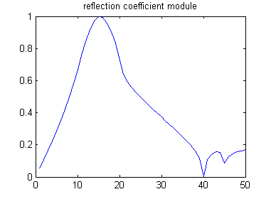
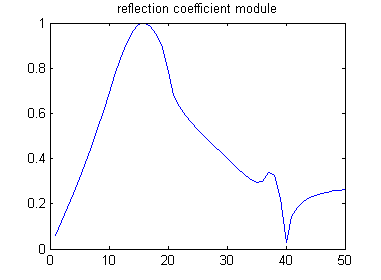
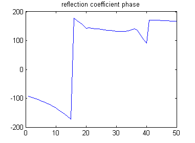
the number of spatial frequencies to M = N = 5 and level of basis functions to P = Q = 4 we obtain the results in the fig. 6.1C.4.
The results in the fig. 6.1C.4 and in the fig. 6.1C.2 are again almost identical, so increasing the number of the spatial frequencies and
level of the basis functions was not necessary. We are trying to use lower numbers of the spatial frequencies and lower levels
of the basis functions to save the computing time. The computing times of analyses are presented in the Tab.1. The computing
time of analysis in the ANSOFT Designer was 149 sec. The similar results was computed in Matlab in 1.6 sec (see fig. 6.1C.2 and fig. 6.1C.3).
We have to consider, that ANSOFT Designer computing all parameters of the FSS for both possible polarizations in the same time.
In the figure are depicted computing times depending on the parameter n = ( M = N = P = Q ) for both types of the basis functions.
The computing times of the basis functions with Chebyshev polynomials are lower then the computing times of the harmonic basis functions.
| Tab. 6.1C.1 | Comparsion of the computing times for harmonic basis functions and for the basis functions with Chebyshev polynomials.
The parameter n is equals M = N = P = Q. The computing time was measured for analysis in the interval (1÷50) GHz with step 1 GHz. |
|
| n [-] |
1 |
2 |
3 |
4 |
5 |
| t [s] (basis functions with Chebyshev polynomials) |
1,6 |
10,4 |
60,8 |
251,5 |
807,5 |
| t [s] (harmonic basis functions) |
1,6 |
10,5 |
62,1 |
268,9 |
908,4 |
|
 |  |
| Obr. 6.1C.2a | Magnitude and angle of the reflection coefficient computed in Matlab with the harmonic basis functions. The parameters of analysis are in the text above. M = N = P = Q = 1 |
|
 |  |
| Obr. 6.1C.2b | Magnitude and angle of the reflection coefficient computed in Matlab with the basis functions with Chebyshev polynomials. The parameters of analysis are in the text above. M = N = P = Q = 1 |
|
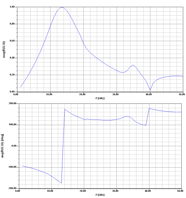 |
| Obr. 6.1C.3 | Magnitude and angle of the reflection coefficient computed in ANSOFT Designer |
|
 |  |
| Obr. 6.1C.4a | Magnitude and angle of the reflection coefficient computed in Matlab with the harmonic basis functions. The parameters of analysis are in the text above. M = N = 5, P = Q = 4 |
|
 |  |
| Obr. 6.1C.4b | Magnitude and angle of the reflection coefficient computed in Matlab with the basis functions with Chebyshev polynomials. The parameters of analysis are in the text above. M = N = 5, P = Q = 4 |
|
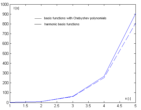 |
| Fig. 6.1C.5 | Comparsion of the computing times of the analyses with the harmonic basis functions with Chebyshev polynomials. |
|
|