(3.1)
3 Optimality conditions - examples
Using examples, we are going to demonstrate the way how can be tested optimality of a given point. For simplicity, we start with a single-variable function, and further, we extent our approach to a two-variable function.
3.1 Single-Variable Function
Assume the following function :
|
(3.1)
|
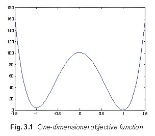
The function is expected to have minims in points x1 = -1, x2 = 0 and x3 = +1. We are aimed to verify it.
First, the stationarity condition has to be verified. Hence, we compute
the first derivative of (3.1)
|
(3.2)
|
 and
we evaluate it for x1,
x2 and x3. Whereas the value of the first
derivative is zero in the first point and in the third one, the value
in the second point equals to -2. Whereas the first-order optimality
condition is met in x1
and x3, in x2
this condition is not met, and the objective function cannot have
minimum in that point.
and
we evaluate it for x1,
x2 and x3. Whereas the value of the first
derivative is zero in the first point and in the third one, the value
in the second point equals to -2. Whereas the first-order optimality
condition is met in x1
and x3, in x2
this condition is not met, and the objective function cannot have
minimum in that point.
In the next step, we have to decide whether the objective function have
minims, maxims or inflexions in x1
and x3. We therefore
compute the second derivative of the objective function
|
(3.3)
|
and evaluate it in points x1
and x3. In both the cases, we come to the value +802.
The positive value of the second derivative proves the minims in the
points x1 and x3.
Correctness of the computation is illustrated by Fig. 3.1, which shows
the function (3.1) near the origin of the coordinate system. We can see
that minims really appear in the points x1
and x3 and that there is a maximum in a small distance
from x2.
3.2 Two-Variable Function
 Assume the following function :
|
(3.4)
|
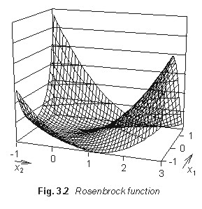
The function (3.4) is called Rosenbrock one. Rosenbrock function
describes a banana-shaped valey of steep slopes in one direction and of
a flat bottom in other direction. From the optimization viewpoint, such
functions are difficult to be minimized, and therefore, Rosenbrock
function is used for testing properties of optimization methods.
Rosenbrock function near the origin of the coordinate system is
depicted in Fig. 3.2.
We are aimed to verify if the minimum of Rosenbrock function is in the
point [1, 1].
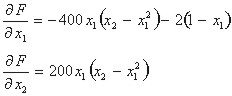
In order to verify the first-order optimality condition, we have to
compute the gradient of the objective function (3.4)
 |
(3.5)
|
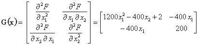
Substituting x1 = 1 and x2 = 1 in (3.5), both the components of the gradient become zero. The norm of the gradient is therefore zero in [1, 1], and hence, we can expect a minimum, a maximum or a saddle point there. In order to decide, which of the three-listed cases corresponds to the point [1,1], we have to compute Hess matrix
 |
(3.6)
|
We substitute x1 = 1 and x2 = 1 to (3.6) and evaluate eigenvalues of Hess matrix in MATLABu using the function eig: k1 = 1001,6 and k2 = 0,4. Both the eigenvalues are positive, Hess matrix is positive definite, and there is a minimum of Rosenbrock function in [1,1].
3.3 When the Derivatives are Unknown ...
 When
solving practical optimization problems, derivatives can be computed
analyticaly in the expected optimal point exceptionally. When designing
an antenna, e.g., its numerical model stays at our disposal in the
computer, which is able to produce a current distribution on antenna
metallic parts and field distribution on antenna apertures for given
frequency and given dimensions of the antenna. In a fact, the numeric
model maps dimesnions as state variables to electric quantities as
parameters of the optimization problem. An analytic expression of the
objective function is not known, and therefore, the gradient and the
Hess matrix have to be computed numerically.
When
solving practical optimization problems, derivatives can be computed
analyticaly in the expected optimal point exceptionally. When designing
an antenna, e.g., its numerical model stays at our disposal in the
computer, which is able to produce a current distribution on antenna
metallic parts and field distribution on antenna apertures for given
frequency and given dimensions of the antenna. In a fact, the numeric
model maps dimesnions as state variables to electric quantities as
parameters of the optimization problem. An analytic expression of the
objective function is not known, and therefore, the gradient and the
Hess matrix have to be computed numerically.
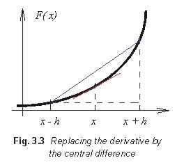
The numeric evaluation of the gradient is based on replacing
derivatives by central differences (Fig. 3.3). When computing the value
of the first derivative in the point x, we are interested in
the direction of the red tangent. Doing a side-step h above
the value x, and a side-step h below the value x,
we create the blue rectangular triangle, which hypotenuse is of the
direction close to the direction of the tangent. The correspondence of
both the directions is better and better when the length of the
side-step h is smaller and smaller. Mathematically, the
substitution of the derivative by the central difference can be
expressed by the following way:
|
(3.7)
|
The eqn. (3.7) shows us, that the length of the side-step cannot be
arbitrarily shortened: when dividing by a very small number, the
numeric error of the computation significantly rises.
When computing a second derivative by central differences, the
computation is divided into two steps:
- using differences, we compute first derivatives in the points x-h
and x+h
|
(3.8)
|
- forming a central difference from (3.8), we create the second
derivative estimate in x.
Working with central differences, we have to carefully consider points,
where the estimate of the derivative is valid.
Now, the above-described method is going to be illustrated by an
example. In the Matlab file rosenbrock.m,
Rosenbrock function (3.4) is stored. The content of the file is assumed
to be unknown, and the file is expected to provide a functional value
on the basis of input parameters x1
and x2 only. We are
again aimed to verify, whether there is the minimum in the point [1,1]
or not.
Let us start with the stationarity condition, and express components of
the gradient using central differences cond01.m:
|
X2(1,1) = rosenbrock( [x(1,1);
x(2,1) + h]); g(1,1) = (X1(1,1) - X1(2,1)) /
(2*h); |
When evaluating the first component of the gradient, we operate the
first variable only, and second variable stays constant. When
evaluating the second component of the gradient, the approach is
similar. Using the side-step h = 10-6,
components of the gradient are smaller than 10-10.
Using the side-step h = 10-8,
components of the gradient are smaller than 10-13.
We can therefore conclude: the norm of the gradient approaches zero
when decreasing the length of the side-step h. Therefore, the
stationarity condition can be considered to be met.
Let's turn our attention to the optimality condition cond02.m:
|
h = 1e-8; X1(1,1) = rosenbrock( [x(1,1) + 2*h; x(2,1)]); f1 = (X1(1,1) - X1(2,1)) / (2*h); G(1,1) = (f1 - f2) / (2*h); X2(1,1) = rosenbrock( [x(1,1); x(2,1) + 2*h]); f1 = (X2(1,1) - X2(2,1)) / (2*h); G(2,2) = (f1 - f2) / (2*h); X3(1,1) = rosenbrock( [x(1,1) + h; x(2,1) + h]); G(1,2) = (X3(1,1) - X3(2,1) - X3(3,1) +
X3(4,1)) / (2*h)^2; g = eig( G); |
In the first two blocks, we compute the second derivative according
to x1, and the second
derivative according to x2.
That way, we obtain the elements G(1,1) and G(2,2) of Hess matrix. The
computation follows the above-descried approach (see eqn. 3.8).
Elements G(1,2) and G(2,1) of Hess matrix are evaluated according to
|
(3.9)
|
When the side-step is set to h = 10-8, the numerical computation provides results, which are identical with the analytical computation.