2 Basic Terms - Examples

Meaning of basic terms from the area of optimization will be illustrated by two examples from the electrical engineering. The first example is devoted to the symmetrical dipole, the second one to the waveguide of the transversal profile H.

2.1 Symmetric dipole

Properties of the symmetric dipole (Fig. 2.1) on a given frequency f are given by its length l and by the radius of the antenna wire a. Those variables can be understood as state ones. The state variables are the elements of the two-dimensional state vector from the real space.

(2.1)

Properties of the symmetric dipole are evaluated from the viewpoint of the input resistance R(l, a) and the input reactance X(l, a). During the optimization, we change values of the length and the radius of the antenna wire such a way to reach the desired values R_d and X_d. The criterial function can be expressed as

(2.2)

Smaller the value of the criterial function is, closer the actual values of the input resistance and the input reactance are to the desired values.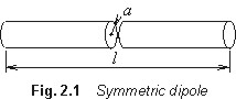

The eqn. (2.2) shows us, why the differences between actual values of input parameters and desired ones are squared. In the opposite case (the differences are not squared), a large positive difference between resistances could compensate a large negative differences between reactances, and the value of the criterial function can be very small even if being in a large distance from the optimum.

If we wish to clasify the criterial function from the viewpoint of the optimization problem clasification (as described in the layer A), we can say the eqn. (2.2) is a sum of squares of non-linear functions (the input resistance and the input reactance depend on the dipole dimensions non-linearly).

When searching such dimensions of the dipole, which are related to the desired impedance on a given frequency, we minimize the criterial function (2.2)

(2.3)

Since the dimensions a and l cannot be negative, we complete the unconstrained optimization (2.3) by constraints

(2.4a)

These constraints are called simple bounds (see the classification of contraints in the layer A).

In order to ensure the antenna to keep the character of the dipole, the antenna length l should be much larger than the antenna radius a (in the opposite case, we get the capacitor with the circular shape of electrodes). If we require the length of the antenna is 100-times larger compared to the radius, we have to add the next constraint

(2.4b)

The condition (2.4b) can be clasified as the linear inequality constraint. The feasible region of the optimization, given by the conditions (2.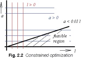4), is depicted in the Fig. 2.2. Optimal values of state variables a and l are not therefore sought over the whole plane [a, l], but we move over the hatched V-shaped area. That way, the space we search for the optimum is significantly reduced.

If we introduce an additional constraint, which limits the maximum dimensions of the antenna, then the feasible region becomes of a finite size. For simplicity, these additional constraints are not introduced here.

Now, we rewrite the whole optimization problem into the matrix, which corresponds to the relations (2.4) in the basic layer.

Simple bounds (2.4a) can be expressed as

(2.5a)

The linear constraint (2.4b) can be rewritten into the form

(2.5b)

Since our constraints are linear, the functions c₁, c₂ and c₃ are of the form of vectors of coefficients c₁ = [0, 1], c₂ = [1, 0] and c₃ = [0.01, -1] .

And this is the end of the first example, which explains the meaning of basic terms from the optimization area.

2.2 H-shaped metallic waveguide

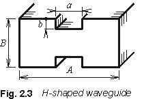Now, we aply all the steps described in the paragraph 2.1 to the formulation of the optimization task related to the metallic waveguide of the H-shaped transversal profile (Fig. 2.3). For simplicity, the waveguide is assummed to be fabricated from the perfect electric conductor (PEC) filled in by the vacuum. We further assume that the waveguide is of the infinite length and its parameters do not change in the longitudinal direction (the wavwguide is said being longitudinally homogeneous). The outer dimensions of the waveguide are identical with the dimension of the waveguide R100, i.e. A = 22.86 mm and B = 10.16 mm. During the optimization, we change the width of the groove a and its height b such way to reach the unimodality of the waveguide in the prescribed frequency band. The unimodal band is given by the critical frequency of the dominant mode TE10 (since this frequency, electromagnetic wave starts to propagate through the waveguide), and by the critical frequency of the second highest mode TE20 (since this frequency, two different waves start to propagate and interfere; the velocity of propagation is different for both the waves).

The criterial function can be formulated as a sum u squared differences between the actual value of the critical frequency of the mode TE10 f₁₀(a, b) and the desired one f_{10, d} , and between the actual value of the critical frequency TE20 f₂₀(a, b) and the desired one f_20,d

(2.6)

From the classification viewpoint, the function (2.6) is the sum of squares of non-linear functions.

The criterial function will be minimized with respect to the groove dimensions a, b

(2.7)

The groove dimensions are arraneged into the form of the state vector

(2.8)

The criterial function is minimized in the two dimensional real state space [a, b]. The state space has to be constrained similarly to the case of the dipole. The groove width a is changed from 0 mm (no groove in the waveguide) to 18 mm (the width of nib of the letter H equals to 4.86 mm). The groove height b can vary from 0 mm (no groove) to 4 mm (the width of the traverse of the letter H is 2.16 mm). Hence, we have simple bounds, which can be expressed by the following matrix form

(2.9)

In case of the H/shaped waveguide, we search the minimum of the criterial function (2.6) in the rectangular feasible region of the finite size 18 mm x 4 mm.

This moment, the optimization task is formulated. Now, we have to only choose an appropriate minimization method, which reveals the optimum in the feasible region. Methods for the unconstrained optimizations (i.e., no constraints are reflected) are describe in the chapter 4.